Multiple object tracking: A literature review
Abstract
Multiple Object Tracking (MOT) has gained increasing attention due to its academic and commercial potential. Although different approaches have been proposed to tackle this problem, it still remains challenging due to factors like abrupt appearance changes and severe object occlusions. In this work, we contribute the first comprehensive and most recent review on this problem. We inspect the recent advances in various aspects and propose some interesting directions for future research. To the best of our knowledge, there has not been any extensive review on this topic in the community. We endeavor to provide a thorough review on the development of this problem in recent decades. The main contributions of this review are fourfold: 1) Key aspects in an MOT system, including formulation, categorization, key principles, evaluation of MOT are discussed; 2) Instead of enumerating individual works, we discuss existing approaches according to various aspects, in each of which methods are divided into different groups and each group is discussed in detail for the principles, advances and drawbacks; 3) We examine experiments of existing publications and summarize results on popular datasets to provide quantitative and comprehensive comparisons. By analyzing the results from different perspectives, we have verified some basic agreements in the field; and 4) We provide a discussion about issues of MOT research, as well as some interesting directions which will become potential research effort in the future.
多目标跟踪(MOT)因其在学术和商业上的巨大潜力而受到越来越多的关注。虽然已经提出了不同的方法来解决这个问题,但由于外观突变和严重的物体遮挡等因素,仍然具有挑战性。在这项工作中,我们贡献了对这个问题的第一次全面和最新的评论期刊。我们综述了近年来在各个方面的研究进展,并对未来的研究提出了一些有趣的方向。据我们所知,社会上并没有就这个课题进行任何广泛的检讨。我们努力对近几十年来这一问题的发展进行彻底的审查。这篇综述的主要贡献有四个方面:1)讨论了MOT系统中的关键方面,包括MOT的制定、分类、关键原则、评估;2)我们不列举个别作品,而是按不同方面讨论现有的方法,每种方法被分成不同的组,详细讨论每一组的原理、优点和缺点;3)我们检查现有出版物的实验,并在流行的数据集上总结结果,以提供定量和全面的比较。通过从不同角度分析研究结果,验证了该领域的一些基本共识;4)对MOT研究的问题进行了讨论,并对未来可能的研究方向进行了展望。
Introduction
Apart from the common challenges in both SOT and MOT, further key issues that complicate MOT include among others:
- Frequent occlusions.
- Initialization and termination of tracks.
- Dimilar appearance.
- Interactions among multiple objects.
In order to deal with all these issues, a wide range of solutions have been proposed in the past decades. These solutions concentrate on different aspects of an MOT system, making it difficult for MOT researchers, especially newcomers, to gain a comprehensive understanding of this problem.== Therefore, in this work we provide a review to discuss the various aspects of the multiple object tracking problem.
Contributions
- We derive a unified formulation of the MOT problem which consolidates most of the existing MOT methods, and two different ways to categorize MOT methods.
- We investigate different key components involved in an MOT system, each of which is further divided into different aspects and discussed in detail regarding its principles, advances, and drawbacks.
- Experimental results on popular datasets regarding different approaches are presented, which makes future experimental comparison convenient. By investigating the provided results, some interesting observations and findings are revealed.
- By summarizing the MOT review, we unveil existing issues of MOT research. Furthermore, open problems are discussed to identify potential future research directions.
- 我们推导出了 MOT 问题的统一公式,该公式整合了大多数现有的 MOT 方法,以及两种不同的 MOT 方法分类方法。
- 我们研究了 MOT 系统中涉及的不同关键组件,每个组件都进一步分为不同的方面,并详细讨论了其原理,优点和缺点。
- 给出了关于不同方法的流行数据集的实验结果,方便了未来的实验比较。通过调查所提供的结果,揭示了一些有趣的观察和发现。
- 通过总结 MOT 的回顾,我们揭示了 MOT 研究的现有问题。此外,还讨论了开放性问题,以确定未来潜在的研究方向。
Denotations
Throughout this manuscript, we denote scalar and vector variables by lowercase letters (e.g., ) and bold lowercase letters (e.g., ), respectively. We use bold capital letters (e.g., ) to denote a matrix or a set of vectors. Capital letters (e.g., ) are adopted for specific functions or variables. Table 2 lists symbols utilized throughout this review. Except the symbols in the table, there may be some symbols for a specific reference. As these symbols are not commonly employed, they are not listed in the table but will be rather defined in the context.
在整篇手稿中,我们分别用小写字母(例如: )和粗体小写字母(例如,)表示标量变量和向量变量。我们使用粗体大写字母(例如,)来表示一个矩阵或一组向量。大写字母(例如,)用于特定的函数或变量。表2列出了本综述中使用的符号。除表中的符号外,可能还有一些符号用于特定引用。由于这些符号不常用,因此它们不会在表中列出,而是在上下文中定义。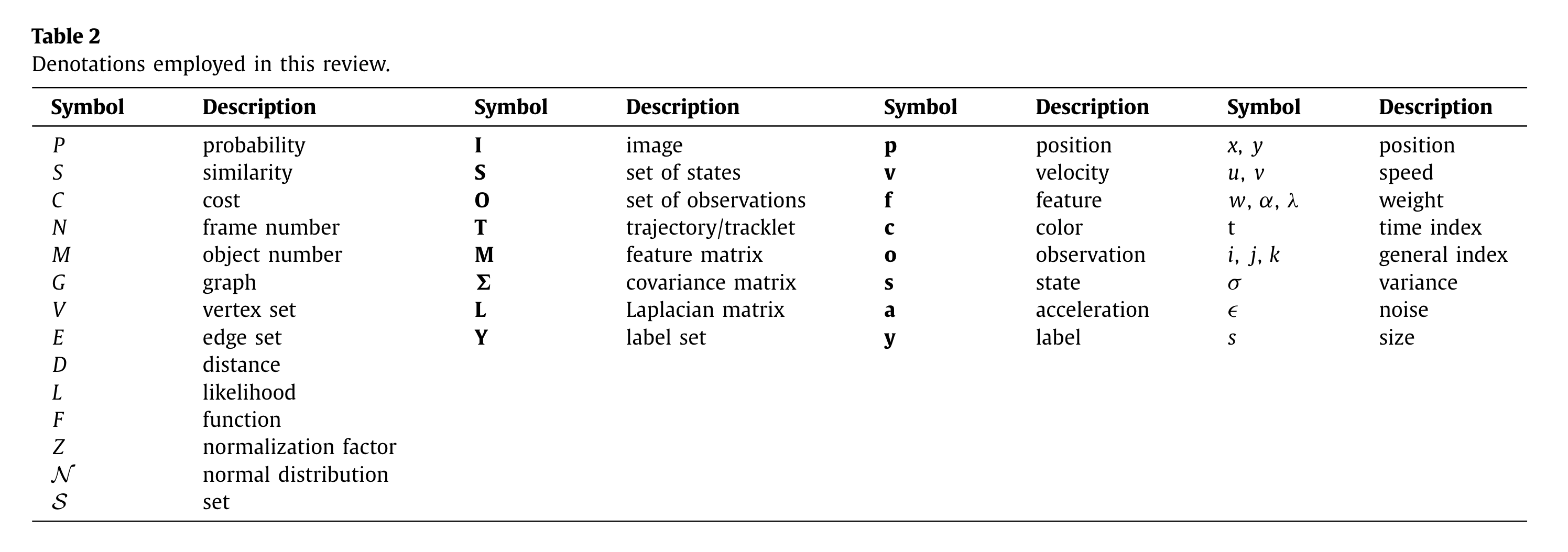
MOT problem
Problem formulation
In general, multiple object tracking can be viewed as a multi-variable estimation problem. Given an image sequence, we employ to denote the state of the -th object in the -th frame, to denote states of all the objects in the -th frame. We employ to denote the sequential states of the -th object, where and are respectively the first and last frame in which target exists, and to denote all the sequential states of all the objects from the first frame to the -th frame. Note that the object number may vary from frame to frame.
Correspondingly, following the most commonly used tracking-by-detection, or Detection Based Tracking (DBT) paradigm, we utilize to denote the collected observations for the -th object in the -th frame, to denote the collected observations for all the objects in the -th frame, and to denote all the collected sequential observations of all the objects from the first frame to the -th frame.
The objective of multiple object tracking is to find the “optimal” sequential states of all the objects, which can be generally modeled by performing MAP (Maximum a posteriori) estimation from the conditional distribution of the sequential states given all the observations:
一般来说,多目标跟踪问题可以看作是一个多变量估计问题。给定图像序列,我们用 来表示第 帧中第 个对象的状态, 表示第 帧中所有 个对象的状态。我们用 来表示第 个对象的序列状态,其中 和 分别是目标 存在的第一帧和最后一帧,并且 表示从第一帧到第 帧所有对象的所有序列状态。请注意,对象编号可能因帧而异。
相应地,遵循最常用的检测跟踪或基于检测的跟踪(DBT)范式,我们利用 来表示为第 帧中的第 个对象收集的观测结果, 表示第 帧中所有 对象的收集观测,并且 表示从第一帧到第 帧收集的所有对象的所有顺序观测。
多目标跟踪的目标是找到所有目标的最优序列状态,这通常可以通过从给定所有观测的序列状态的条件分布执行 MAP(最大后验概率)估计来建模:
Different MOT algorithms from previous works can now be thought as designing different approaches to solving the above MAP problem, either from a probabilistic inference perspective or a deterministic optimization perspective.
The probabilistic inference based approaches usually solve the MAP problem in Eq. (1) using a two-step iterative procedure as follows,
,
.
Here and are the Dynamic Model and the Observation Model, respectively.
The deterministic optimization based approaches directly maximize the likelihood function as a delegate of over a set of available observations :
与以前工作不同的 MOT 算法现在可以被认为是设计了不同的方法来解决上述 MAP 问题,无论是从概率推理角度还是从确定性优化角度。
基于概率推理的方法通常使用两步迭代过程来等式 (1) 中的 MAP 问题,如下所示:
,
.
这里, 和 分别是动态模型和观测模型。
基于确定性优化的方法直接将似然函数 最大化,作为 的代表,覆盖一组可用观测 :
or conversely minimize an energy function :
或者反过来最小化能量函数 :
where is a normalization factor to ensure to be a probability distribution.
其中, 是确保 服从概率分布的归一化因子。
MOT categorization
In the following we attempt to conduct this according to three criteria:
- initialization method
- processing mode
- type of output
Initialization method
Most existing MOT works can be grouped into two sets, depending on how objects are initialized:
- Detection-Based Tracking (DBT)
- Detection-Free Tracking (DFT)
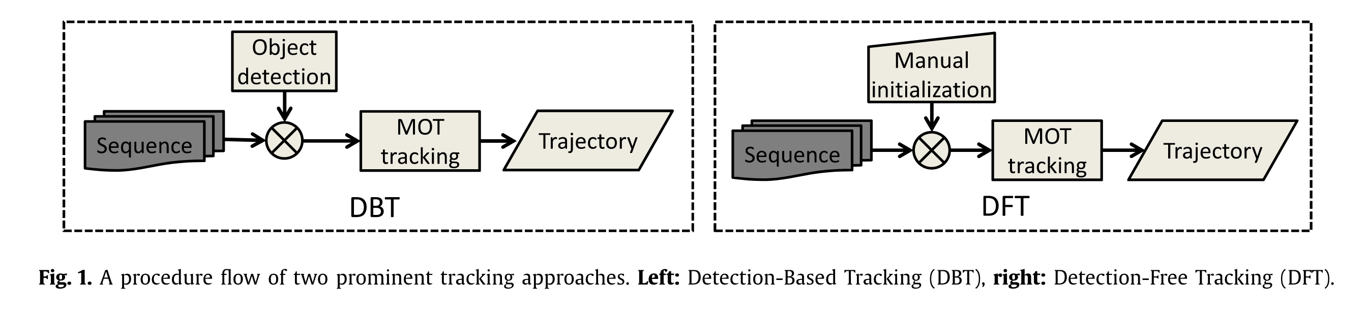
Detection-based tracking
Objects are first detected and then linked into trajectories. This strategy is also commonly referred to as "tracking-by-detection". Given a sequence, type-specific object detection or motion detection (based on background modeling) is applied in each frame to obtain object hypotheses, then (sequential or batch) tracking is conducted to link detection hypotheses into trajectories. There are two issues worth noting. First, since the object detector is trained in advance, the majority of DBT focuses on specific kinds of targets, such as pedestrians, vehicles or faces. Second, the performance of DBT highly depends on the performance of the employed object detector.
首先检测对象,然后将其链接到轨迹中。这种策略通常也被称为“检测跟踪”。给定一个序列,在每帧中应用特定类型的目标检测或运动检测(基于背景建模)以获得目标假设,然后进行(序列或批量)跟踪以将检测假设链接到轨迹中。有两个问题值得注意。首先,由于目标检测器是预先训练的,因此大多数 DBT 都集中在特定类型的目标上,例如行人、车辆或人脸。其次,DBT 的性能高度依赖于所采用的对象检测器的性能。
Detection-free tracking
DFT requiresmanual initialization of a fixed number of objects in the first frame, then localizes these objects in subsequent frames.
DFT 要求在第一帧中手动初始化固定数量的对象,然后在后续帧中定位这些对象。
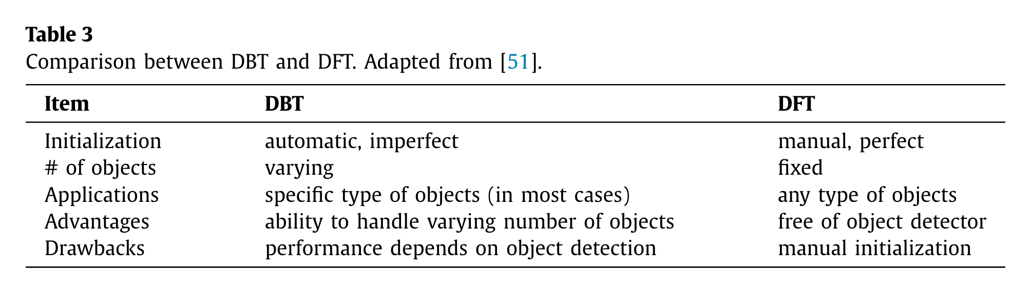
DBT is more popular because new objects are discovered and disappearing objects are terminated automatically. DFT cannot deal with the case that objects appear. However, it is free of pre-trained object detectors. Table 3 lists the major differences between DBT and DFT.
DBT 更受欢迎,因为新的对象被发现,消失的对象被自动终止。DFT 不能处理对象出现的情况。然而,它没有经过预先训练的物体探测器。表3列出了 DBT 和 DFT 之间的主要区别。
Processing mode
MOT can also be categorized into:
- Online tracking.
- Offline tracking.
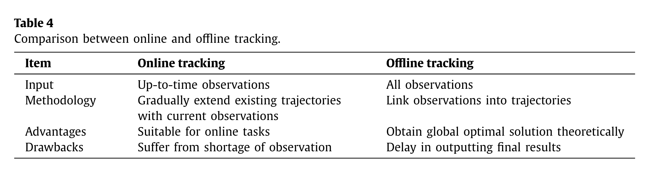
The difference is whether observations from future frames are utilized when handling the current frame. Online, also called causal, tracking methods only rely on the past information available up to the current frame, while offline, or batch tracking approaches employ observations both in the past and in the future.
Online tracking
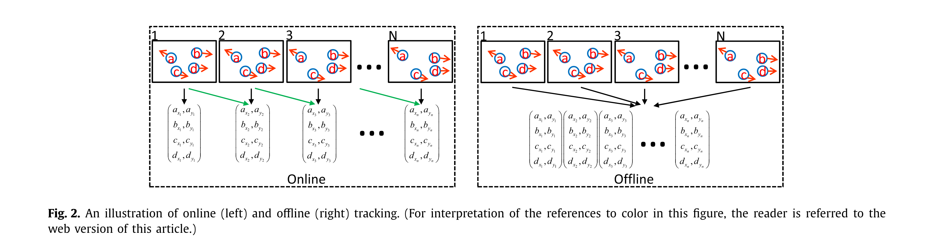
In online tracking, the image sequence is handled in a step-wise manner, thus online tracking is also named as sequential tracking. An illustration is shown in Fig. 2 (top), with three objects (different circles) a, b, and c. The green arrows represent observations in the past. The results are represented by the object’s location and its ID. Based on the up-to-time observations, trajectories are produced on the fly.
在在线跟踪中,对图像序列进行分步处理,因此在线跟踪也称为顺序跟踪。图2(上图)显示了三个物体(不同的圆圈)a、b 和 c。绿色箭头表示过去的观测结果。结果由物体的位置和 ID 表示。基于最新的观察,动态地产生轨迹。
Offline tracking
Offline tracking utilizesa batch of frames to process the data. As shown in Fig. 2 (bottom), observations from all the frames are required to be obtained in advance and are analyzed jointly to estimate the final output. Note that, due to computational and memory limitation, it is not always possible to handle all the frames at once. An alternative solution is to split the data into shorter video clips, and infer the results hierarchically or sequentially for each batch. Table 4 lists the differences between the two processing modes.
离线跟踪利用一批帧来处理数据。如图2(下图)所示,所有帧的观测值都需要预先获得,并联合分析以估计最终输出。请注意,由于计算和内存限制,一次处理所有帧并不总是可能的。另一种解决方案是将数据分割成较短的视频剪辑,并分层或按顺序推断每一批的结果。表4列出了两种处理模式之间的差异。
Type of output
This criterion classifies MOT methods into deterministic ones and probabilistic ones, depending on the randomness of output. The difference between these two types of methods primarily results from the optimization methods adopted as mentioned in Section 2.1.
Stochastic tracking
The output results of stochastic tracking vary from time to time. For example, in the case of detection-free tracking, the bounding box results are different if we utilize particle filter for inference. The difference results from the randomness of the generation of particles in the processing. Even in the case of detection-based tracking, some studies also employ state-of-the-art single object tracker to refine the detection bounding boxes. This kind of methods will also lead to different tracking results in different running times.
随机跟踪的输出结果随时间的变化而变化。例如,在无检测跟踪的情况下,如果使用粒子滤波进行推理,则边界框结果不同。这种差异是由于加工过程中产生的颗粒的随机性造成的。即使在基于检测的跟踪的情况下,一些研究也使用了最先进的单目标跟踪器来优化检测边界框。这种方法在不同的运行时间也会导致不同的跟踪结果。
Deterministic tracking
The output of deterministic tracking is constant when running the methods multiple times. For instance, in the case of tracking-by-detection, data association methods like Hungarian algorithm will produce deterministic tracking results. Deterministic tracking usually is associated with deterministic optimization for deriving the final output.
当多次运行这些方法时,确定性跟踪的输出是恒定的。例如,在检测跟踪的情况下,匈牙利算法等数据关联方法将产生确定性的跟踪结果。确定性跟踪通常与用于导出最终输出的确定性优化相关联。
Discussion
The difference between DBT and DFT is whether a detection model is adopted (DBT) or not (DFT). The key to differentiate online and offline tracking is the way they process observations. Readers may question whether DFT is identical to online tracking because it seems DFT always processes observations sequentially. This is true in most cases although some exceptions exist. Orderless tracking is an example. It is DFT and simultaneously processes observations in an orderless way. Though it is for single object tracking, it can also be applied for MOT, and thus DFT can also be applied in a batch mode. Another vagueness may rise between DBT and offline tracking, as in DBT tracklets or detection responses are usually associated in a batch way. Note that there are also sequential DBT which conducts association between previously obtained trajectories and new detection responses.
DBT 和 DFT 的区别在于是否采用检测模型(DBT)或不采用检测模型(DFT)。区分线上和线下跟踪的关键是它们处理观测的方式。读者可能会质疑 DFT 是否等同于在线跟踪,因为 DFT 似乎总是按顺序处理观察结果。这在大多数情况下都是正确的,尽管也有一些例外。无序跟踪就是一个例子。它是 DFT,同时以一种无序的方式处理观测数据。虽然它是用于单目标跟踪的,但它也可以应用于 MOT,因此 DFT 也可以批量应用。在 DBT 和离线跟踪之间可能会出现另一种模糊,因为在 DBT 跟踪小程序或检测响应中通常以批处理的方式相关联。注意,还存在在先前获得的轨迹和新的检测响应之间进行关联的顺序 DBT。